Interacting with Pulsar Data
Overview
Teaching: 60 min
Exercises: 30 minQuestions
How do I inspect my pulsar data
How can I remove RFI from my observations
Objectives
Learn the software used to process pulsars
Introduction
In this lesson we will go over how to interact with pulsar data. We will go over the different types of data, how to plot them and how to clean them.
The data we will use for this lesson can be downloaded with the following command:
wget "ftp://elwood.ru.ac.za/pub/geyer/NWU_pulsartiming/data/Session1_pulsar_data.tar.gz"
Then untar it with
tar -xvf Session1_pulsar_data.tar.gz
And move into the directory it creates with
cd pulsar_data_lesson
Pulsar data types
Pulsar data are typically stored as a three-dimensional array of pulse profiles the axes being time (sub-integrations), observing frequency (channels) and polarization. Each data file (typically termed as archives) have attributes (metadata) that describe the pulsar observation. Pulsar data can be broadly sorted into two types, “raw voltage” which is the time series data as it comes off the telescope and “folded” which has been folded and dedisperesed using a timing ephemeris.
Some formats for raw voltage files include PSRFITS, PSRDADA and VDIF.
Before analyzing the data you often have to fold and dedisperse the data which is often done with dspsr (explained in the next section).
The folded data are often called archives and have .ar at the end of their filename.
Many telescopes (such as MeerKAT) have a pulsar timing backend that will automatically produce a folded archive to save processing and data size.
DSPSR
DSPSR is not installed on the VM or need for MeerKAT data but it is still useful to know how to use to process other data and to understand MeerKAT data.
dspsr can perform phase-coherent dispersion removal while folding the data based on the input ephemeris.
The output data may be divided into sub-integrations of arbitrary length, including single pulses.
THe MeerKAT PTUSE outputs the archives in ~8 second sub-integrations so the equivalent dspsr command may look like this:
dspsr -F 128 -E 1644-4559.eph -L 8 raw_observation.data
where -F 128 outputs a 128 frequency channel archive, -E 1644-4559.eph is the ephemeris file, -L 8 outputs an archive for every 8 seconds of data and raw_observation.data is whatever the input raw voltage file is called (if there is one).
Because these archives have already been folded with an ephemeris, there is only so much you can do to improve your observation if the ephemeris is inaccurate. For example below is a recent observation (2023-04-21-23:58:20) of PSR J1705-1903’s profile and phase against time plots:
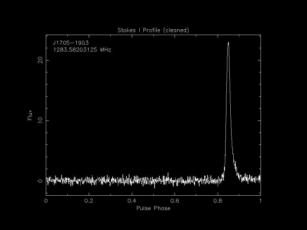
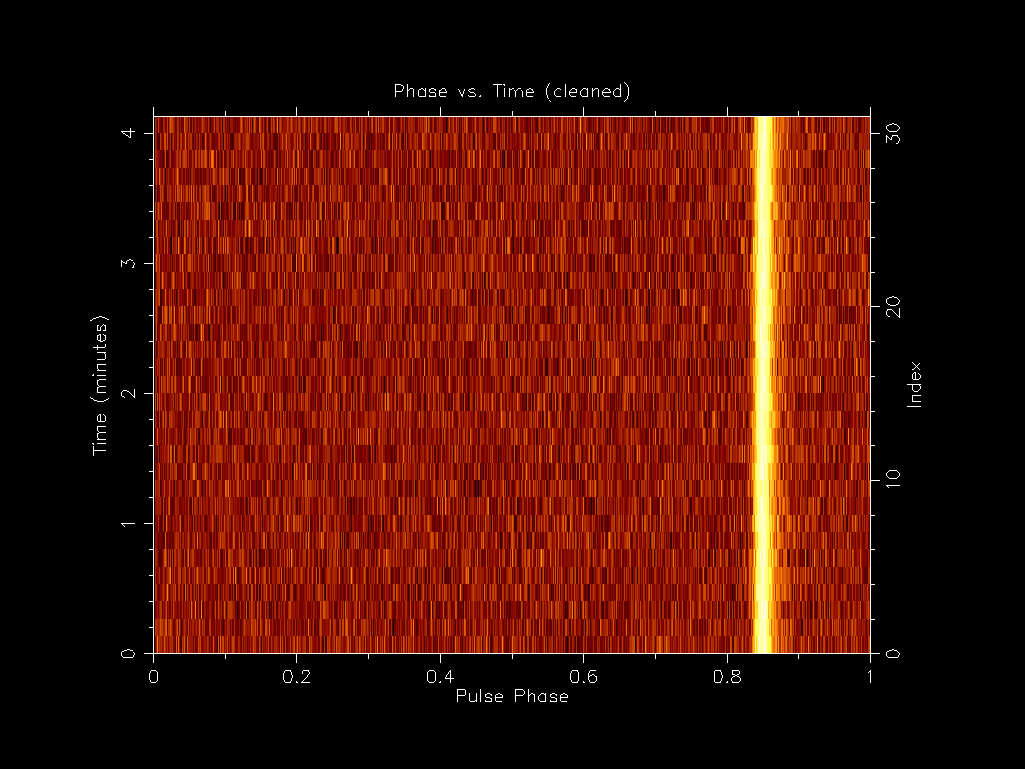
You can see that pulse is thin as expected. If we then compare this to an early observation (2019-04-23-05:44:10) we can see that the pulse profile is much wider even though we have a applied a more recent ephemeris to it.
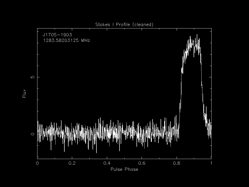
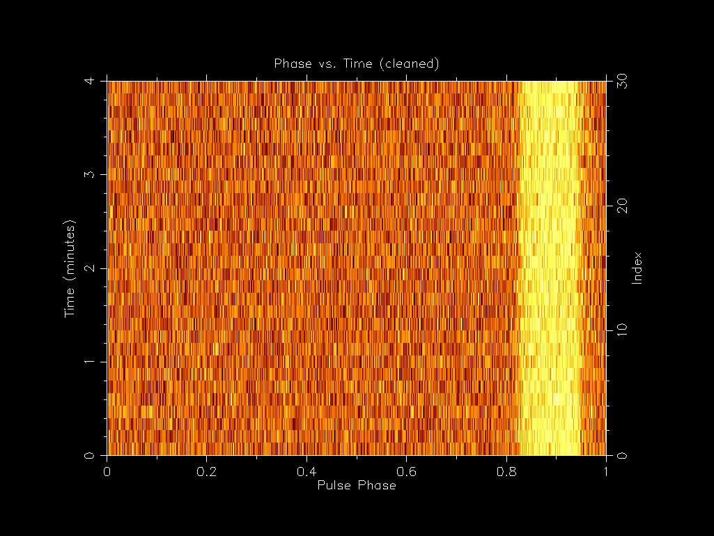
This is due to the PTUSE outputting the 8 second sub-integrations which have some timing smear in them due to the initial inaccurate ephemeris used during the observation. If you ever want to inspect the ephemeris used to create an archive file you can use the following command:
vap -E <archive_file>
PSRCHIVE
Now that we have folded and dedisperesed archives, we can analysis them and one of the best packages to do that is PSRCHIVE. PSRCHIVE is an Open Source C++ development library for the analysis of pulsar astronomical data. The software is described online and in Hotan, van Straten & Manchester (2004) and Straten, Demorest & Osłowski 2012.
There is a full list of commands online and below are the most common ones:
psrstatquery attributes and statisticspsraddcombine data in various wayspsrplotproduce customized, publication quality plotsvapoutput tables of parameters and derived valuespavproduce a wider variety of plotspamcommand line general purpose data reductionrmfitestimate the Faraday rotation measurepasgenerate template profiles (standards)patproduce time of arrival estimatespazRFI mitigationpdmpfind optimal period and dispersion measure
Investigating files (vap and psrstat)
Archive files have a lot of metadata associated with them and you can use the vap and psrstat command to view them.
The main difference between the two is that vap outputs the metadata in a table format and psrstat outputs it in a more human readable format and includes more statistics.
Lets look at the metadata of one of the archives we will be using for this lesson.
First lets look at the vap output:
vap -c nchan,nsub,length J1903-7051_2022-07-17-22:44:02_*.ar
filename   nchan   nsub   length
J1903-7051_2022-07-17-22:44:02_raw.ar   1024   31   248.000
J1903-7051_2022-07-17-22:44:02_zap.ar   1024   31   248.000
psrstat -c nchan,nsubint,length J1903-7051_2022-07-17-22:44:02_*.ar
J1903-7051_2022-07-17-22:44:02_raw.ar nchan=1024 nsubint=31 length=248
J1903-7051_2022-07-17-22:44:02_zap.ar nchan=1024 nsubint=31 length=248
You’ll notice that they output the values in different formats and that they label the time sub-integrations differently (nsub vs nsubint).
The psrstat command also has access to more statistics and you can output all of the by not including the -c option:
psrstat J1903-7051_2022-07-17-22:44:02_zap.ar
Output
file Name of the file J1903-7051_2022-07-17-22:44:02_zap.ar nbin Number of pulse phase bins 1024 nchan Number of frequency channels 1024 npol Number of polarizations 4 nsubint Number of sub-integrations 31 type Observation type Pulsar site Telescope name MeerKAT name Source name J1903-7051 coord Source coordinates 19:03:38.794-70:51:43.46 freq Centre frequency (MHz) 1283.58203125 bw Bandwidth (MHz) 856 dm Dispersion measure (pc/cm^3) 19.6599998474121 rm Rotation measure (rad/m^2) 18.9939160066885 dmc Dispersion corrected 0 rmc Faraday Rotation corrected 0 polc Polarization calibrated 0 scale Data units FluxDensity state Data state Coherence length Observation duration (s) 248 int*:@ int:help for attribute list ext:obs_mode Observation Mode PSR ext:obsfreq Centre frequency 1283.58203125 ext:obsbw Bandwidth 856 ext:obsnchan Number of channels 1024 ext:hdrver Header Version 6.7 ext:date File Creation Date 2023-09-06T11:14:39 ext:coord_md Coordinate mode J2000 ext:equinox Coordinate equinox 2000 ext:trk_mode Tracking mode TRACK ext:bpa Beam position angle 0 ext:bmaj Beam major axis 0 ext:bmin Beam minor axis 0 ext:stt_date Start UT date 2022-07-17 ext:stt_time Start UT 22:44:02 ext:stt_imjd Start MJD 59777 ext:stt_smjd Start second 81851 ext:stt_offs Start fractional second 0.996758526449667 ext:stt_lst Start LST 0 ext:stt_crd1 Start coord 1 19:03:38.7935 ext:stt_crd2 Start coord 2 -70:51:43.461 ext:stp_crd1 Stop coord 1 19:03:38.7935 ext:stp_crd2 Stop coord 2 -70:51:43.461 ext:ra Right ascension 19:03:38.794 ext:dec Declination -70:51:43.461 obs:observer Observer name(s) Ryan obs:projid Project name SCI-20180516-MB-05 itrf:ant_x ITRF X coordinate. 5109360.133 itrf:ant_y ITRF Y coordinate. 2006852.586 itrf:ant_z ITRF Z coordinate. -3238948.127 rcvr:name Receiver name KAT rcvr:basis Basis of receptors lin rcvr:hand Hand of receptor basis -1 rcvr:sa Symmetry angle of receptor basis 45deg rcvr:rph Reference source phase 0deg rcvr:fdc Receptor basis corrected 1 rcvr:prc Receptor projection corrected 1 rcvr:ta Tracking angle of feed 0deg be:name Name of the backend instrument MKBF be:phase Phase convention of backend +1 be:dcc Downconversion conjugation corrected 0 be:phc Phase convention corrected 0 be:delay Backend propn delay from digi. input. 0 be:config Configuration filename be:nrcvr Number of receiver channels 2 be:tcycle Correlator cycle time 8 hist:nrow Number of rows in history 12 hist:nbin_prd Nr of bins per period 1024 hist:tbin Time per bin or sample 3.51344981959837e-06 hist:chan_bw Channel bandwidth 0.8359375 hist:cal_file Calibrator filename NONE aux:dm_model Auxiliary dispersion model NONE aux:dmc Auxiliary dispersion corrected 0 aux:rm_model Auxiliary birefringence model NONE aux:rmc Auxiliary birefringence corrected 0 sub:int_type Time axis (TIME, BINPHSPERI, BINLNGASC, etc) TIME sub:int_unit Unit of time axis (SEC, PHS (0-1), DEG) SEC sub:tsamp [s] Sample interval for SEARCH-mode data 0 sub:nbits Nr of bits/datum (SEARCH mode 'X' data, else 1) -1 sub:nch_strt Start channel/sub-band number (0 to NCHAN-1) -1 sub:nsblk Samples/row (SEARCH mode, else 1) 1 sub:nrows Nr of rows in subint table (search mode) 31 sub:zero_off Zero offset for SEARCH-mode data 0 sub:signint 1 for signed ints in SEARCH-mode data, else 0 0 subint Sub-integration index 0 chan Frequency channel index 0 pol Polarization index 0 include[:@] Estimator of included bins exclude[:@] Estimator of excluded bins on[:@] On-pulse estimator consecutive:{threshold=3,consecutive=3} on:count Count of selected phase bins 0 on:start Start of the phase region on:end End of the phase region on:min minimum value nan on:max maximum value nan on:range range of values nan on:sum sum of values nan on:avg average of values nan on:rms standard deviation of values nan on:mu3 skewness of values nan on:mu4 kurtosis of values nan on:dev coefficient of deviation of values nan on:med median of values nan on:mdm median absolute difference from median nan on:iqr inter-quartile range of values nan on:qcd quartile coefficient of dispersion nan on:qcs quartile coefficient of skewness nan on:ock octile coefficient of kurtosis nan on:ft1 first harmonic of values nan on:ftN last harmonic of values nan on:mh2 maximum harmonic in upper half-spectrum nan on:ftm median harmonic in upper half-spectrum nan on:sm2 total power in upper half-spectrum nan on:sm3 skew of upper half-spectrum nan on:sm4 kurtosis of upper half-spectrum nan on:sho sum of harmonic outlier power nan on:sdo sum of detrended outlier power nan on:fte spectral entropy nan on:cbp best-fit phase of cyclic box car nan off[:@] Off-pulse estimator minimum:{smooth[:@]=mean:{width=0.150000005960464},find_min=1,find_mean=0,search=0:0,found=0.0929687470197678:0.242968752980232} off:count Count of selected phase bins 154 off:start Start of the phase region 95 off:end End of the phase region 248 off:min minimum value 684.793518066406 off:max maximum value 733.203979492188 off:range range of values 48.4104614257812 off:sum sum of values 109085.38885498 off:avg average of values 708.346680876497 off:rms standard deviation of values 8.90468957888328 off:mu3 skewness of values 0.00585555706206417 off:mu4 kurtosis of values 2.82917703966072 off:dev coefficient of deviation of values 0.0125710895798435 off:med median of values 708.860107421875 off:mdm median absolute difference from median 6.20037841796875 off:iqr inter-quartile range of values 13.1571655273438 off:qcd quartile coefficient of dispersion 0.00928900443988446 off:qcs quartile coefficient of skewness -0.0985447679839679 off:ock octile coefficient of kurtosis 1.10618508398781 off:ft1 first harmonic of values 10.8299932479858 off:ftN last harmonic of values 23.8169898986816 off:mh2 maximum harmonic in upper half-spectrum 268.957733154297 off:ftm median harmonic in upper half-spectrum 51.8983421325684 off:sm2 total power in upper half-spectrum 5510.18733417172 off:sm3 skew of upper half-spectrum -0.297201795034637 off:sm4 kurtosis of upper half-spectrum 2.49651352866569 off:sho sum of harmonic outlier power 0 off:sdo sum of detrended outlier power 3508.27220403776 off:fte spectral entropy 3.30974334238639 off:cbp best-fit phase of cyclic box car 0.38961038961039 all:count Count of selected phase bins 1024 all:start Start of the phase region all:end End of the phase region all:min minimum value 681.297607421875 all:max maximum value 740.071960449219 all:range range of values 58.7743530273438 all:sum sum of values 727073.934204102 all:avg average of values 710.033138871193 all:rms standard deviation of values 8.73123854615207 all:mu3 skewness of values 0.0212097780209406 all:mu4 kurtosis of values 3.03962717627088 all:dev coefficient of deviation of values 0.0122969451257345 all:med median of values 710.058044433594 all:mdm median absolute difference from median 5.86480712890625 all:iqr inter-quartile range of values 11.6577758789062 all:qcd quartile coefficient of dispersion 0.00820995363549673 all:qcs quartile coefficient of skewness -0.0137014989450317 all:ock octile coefficient of kurtosis 1.30218166397035 all:ft1 first harmonic of values 142.131988525391 all:ftN last harmonic of values 21.0218658447266 all:mh2 maximum harmonic in upper half-spectrum 440.245025634766 all:ftm median harmonic in upper half-spectrum 52.1071815490723 all:sm2 total power in upper half-spectrum 35968.0589712215 all:sm3 skew of upper half-spectrum 0.0211442316706619 all:sm4 kurtosis of upper half-spectrum 3.48672406277501 all:sho sum of harmonic outlier power 54.2748589515686 all:sdo sum of detrended outlier power 23408.4130098559 all:fte spectral entropy 4.79931536212596 all:cbp best-fit phase of cyclic box car 0.6005859375 width[:@] Pulse width (turns) 0 snr[:@] Signal-to-noise ratio 5.83387851715088 sumI Total flux in on-pulse phase bins 0 sumP Total polarized flux of on-pulse phase bins 0 sumL Total linearly polarized flux of on-pulse phase bins 0 sumV Total Stokes V of on-pulse phase bins 0 sumC Total circularly polarized flux |V| of on-pulse phase bins 0 sumS Total coherency matrix determinant of on-pulse phase bins 0 varL Variance of the off-pulse linearly polarized flux 144.241568624316 peak Phase of pulse peak (turns) 0.5703125 weff Effective pulse width (turns) -nan nfnr Noise-to-Fourier-noise ratio 1.06242525577545 ncal Number of CAL transitions 0 d2bit 2-bit distortion 0 wtfreq Weighted frequency 1288.502 bwidth Phase bin width 3.51344981959837e-06 dsmear Dispersive smearing in worst channel 0.000217444879083687
Which is nice and verbose, explaining what each attribute is, but is large and perhaps a bit overwhelming.
Making plots
One of the best commands to make plots is psrplot.
You can list all the types of plots that you can make with
psrplot -P
Available Plots:
flux      [D]  Single plot of flux
stokes    [s]  Stokes parameters
Scyl      [S]  Stokes; vector in cylindrical
Scyl+     [E]  Stokes; vector in cylindrical+
Ssph      [m]  Stokes; vector in spherical
Sfluct    [U]  Stokes; fluctuation power spectra
Sflph     [u]  Stokes; fluctuation phase spectra
freq      [G]  Phase vs. frequency image of flux
freq+     [F]  freq + integrated profile and spectrum
time      [Y]  Phase vs. time image of flux
pa        [o]  Orientation (Position) angle
ell       [e]  Ellipticity angle
p3d       [P]  Stokes vector in Poincare space
pahist    [h]  Phase-resolved position angle histogram
pahist+   [H]  Phase-resolved PA histogram and total profile
psd       [b]  Pulsed power spectrum
2bit      [2]  Two-bit distribution
cal       [C]  Calibrator Spectrum
calm      [M]  Calibrator model information
calp      [p]  Calibrator parameter
line      [R]  Line phase subints
dspec     [j]  Dynamic S/N spectrum
dstat     [d]  Dynamic statistic spectrum
offdspec  [r]  Dynamic baseline spectrum
dcal      [l]  Calibrator dynamic spectrum
dweight   [w]  Weights dynamic spectrum
snrspec   [n]  S/N ratio
calphvf   [X]  Calibrator phase vs frequency plot
bandpass  [B]  Display original bandpass
chweight  [c]  Display Channel Weights
bpcw      [J]  Plot off-pulse bandpass and channel weights
digstats  [K]  Digitiser Statistics
digcnts   [A]  Digitiser Counts histogram
fourth    [4]  4x4 covariance of Stokes parameters
cross     [x]  1-D cross covariances between Stokes parameters
alt       [a]  Greyscale of auxiliary profiles
Some of the common types we will go over soon.
First we should explain some of the other psrplot commands.
You can preprocess the archives before plotting with the -j option.
The pre-processing is done with the psrsh command and you can find the full list of options with psrsh -H.
The following commands are the most common ones:
TTime scrunch to one subintFFrequency scrunch to one channelpPolarisation scrunch to total intensityDDedisperse (but not fscrunch)STransform to Stokes parameters For example-jTFDpwill dedisperse and time, frequency and polarisation scrunch.
You can define how to output the plot with the -D option so you could output the plot as a png with -D output_name.png/png.
Pulse profile
Lets give it a go and try to make a pulse profile plot with the command:
psrplot -p flux -jFTDp -D J1903-7051_profile_fts.png/png J1903-7051_2022-07-17-22:44:02_zap.ar
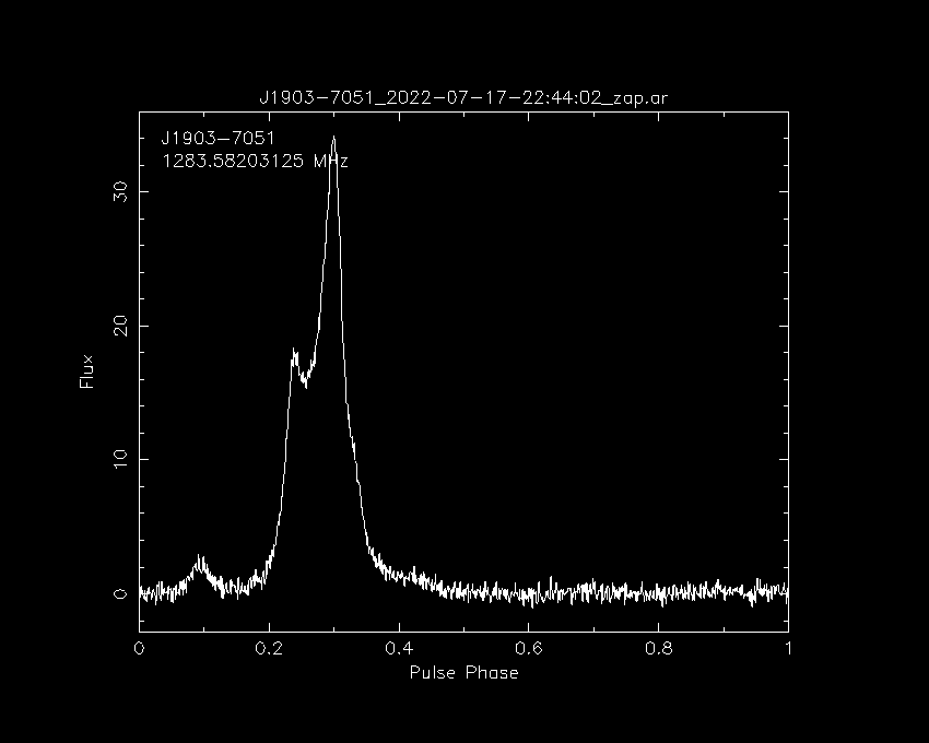
You can also remove the -D J1903-7051_profile_fts.png/png part and it will open the plot in a window.
Now lets go through all the common plot type commands
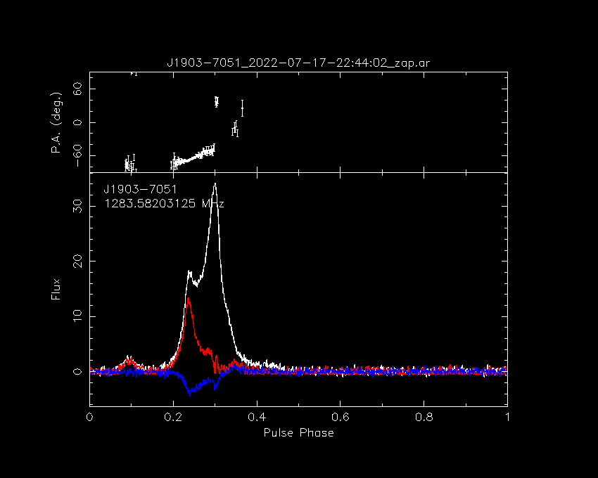
Polarisation (Stokes) profile
psrplot -p Scyl -jFTD -D \J1903-7051_profile_ftp.png/png J1903-7051_2022-07-17-22:44:02_zap.ar
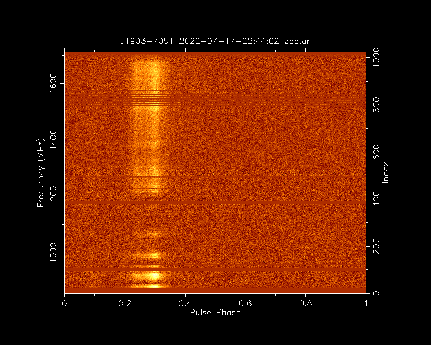
Phase vs. Frequency
psrplot -p freq -jTDp -D J1903-7051_phase_freq.png/png J1903-7051_2022-07-17-22:44:02_zap.ar
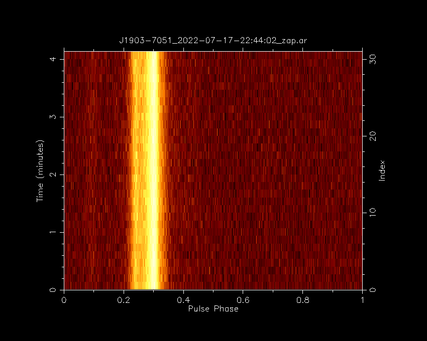
Phase vs. Time
psrplot -p time -jFDp -D J1903-7051_phase_time.png/png J1903-7051_2022-07-17-22:44:02_zap.ar
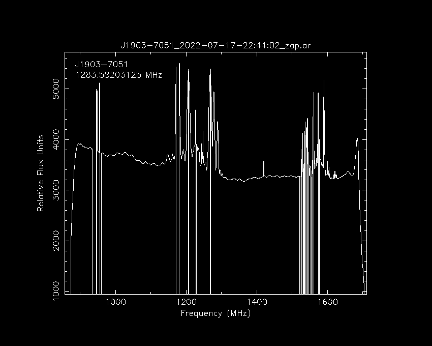
Cleaned bandpass
psrplot -p b -jT -D J1903-7051_bandpass.png/png J1903-7051_2022-07-17-22:44:02_zap.ar
RFI cleaning
While most telescopes are situated in radio quiet zones, it is impossible to remove all sources of RFI.
For this reason, it is important to remove RFI from your data before analysis.
The J1903-7051_2022-07-17-22:44:02_zap.ar archive has already been RFI cleaned and we can see in the bandpass which frequencies were flagged:
We have a uncleaned file that we can use the different technquies on to do our best to clean the archive.
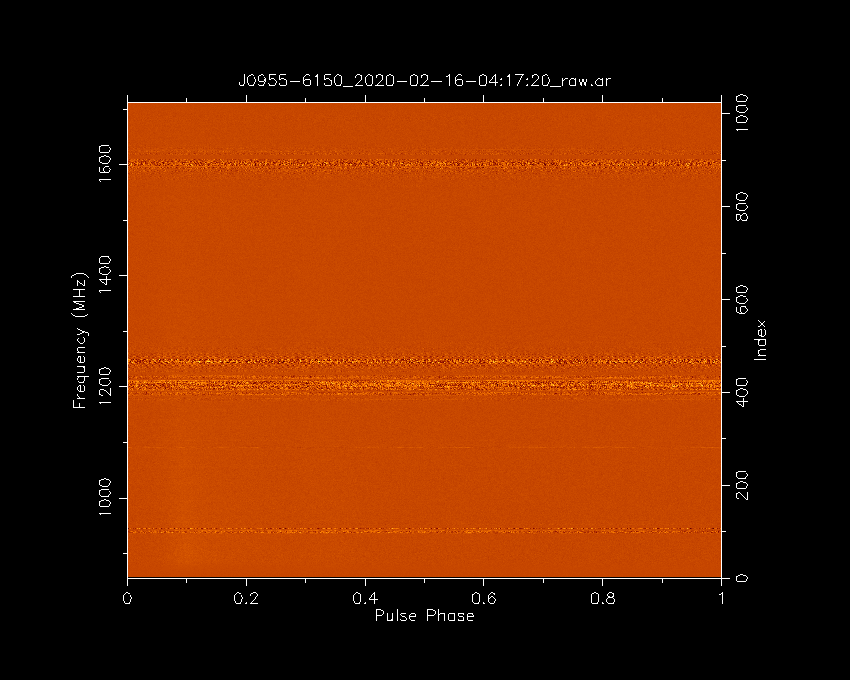
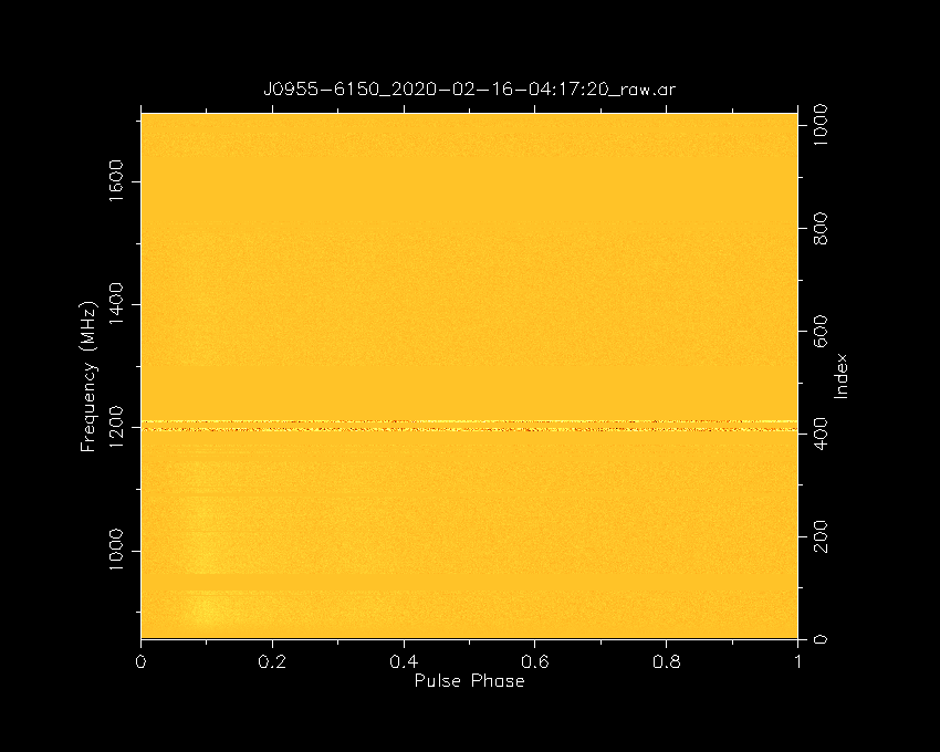
We will be using J0955-6150_2020-02-16-04:17:20_raw.ar as our example file which has signifficant RFI in it which we can when we plot it with the following command:
psrplot -p freq -jTDp -D J0955-6150_phase_freq_raw.png/png J0955-6150_2020-02-16-04:17:20_raw.ar
Paz
paz is a psrchive command that can do some automated and manual RFI removal.
You can use it manually or as a part of other commands.
What I mean by manually is you can use it to create a new archive with a command like so:
paz -r -e paz_median J0955-6150_2020-02-16-04\:17\:20_raw.ar
where -r zap channels using median smoothed difference and -e paz_median outputs a new file ending in .paz_median.
You can then plot this with the following command:
psrplot -p freq -jTDp -D J0955-6150_phase_freq_median.png/png J0955-6150_2020-02-16-04:17:20_raw.paz_median
Or I can produce the same result by addind the ,"zap median to the psrplot command to do this in one go (note that I’m using the original .ar file)
psrplot -p freq -jTDp,"zap median" -D J0955-6150_phase_freq_median.png/png J0955-6150_2020-02-16-04:17:20_raw.ar
Both of these methods will create the following output:
As you can see it removed enough RFI that we can now see the pulsar but there is still some major RFI that was missed.
Pazi
For interactive RFI removal we can use pazi which will create a window where we can select which frequency or time range we wish to flag.
If we run the pazi command with no options it will output the following help:
pazi

A user-interactive program for zapping subints, channels and bins.
Usage: pazi [filename]

Options.
  -h                         This help page.

Mouse and keyboard commands.
  zoom:                      left click, then left click
  reset zoom:                'r'

Modes:
  phase-vs-frequency:        'f'
  phase-vs-time:             't'
  binzap-integration:        'b' (must be in phase-vs-time mode)

  center pulse:              'c'
  toggle dedispersion:       'd'

  zap:                       right click
  zap (multiple):            left click, then right click
  undo last:                 'u'

  In binzap mode:
    -  zoom and reset zoom as above
    -  zap phase range:      left click, then right click
    -  mow the lawn:         'm'
    -  prune the hedge:      'x' to start box, 'x' to finish

  save (<filename>.pazi):    's'
  quit:                      'q'
  print paz command:         'p'
You’ll want to run pazi <file_name> then click f to go to phase-vs-frequency mode then left click and the start of a frequency range then right click and the end of the range that you want to zap.
When you are done press s and q and it will make a new file ending in .pazi.
Remove as much RFI as you can
You can estimate the signal-to-noise ratio of an archive with the following command
psrstat -j FTp -c snr=pdmp -c snr <archive_file_here>Try using pazi to remove as much RFI as you can which keeping the S/N high. Whoever gets the highest S/N wins!
PDMP
pdmp is a tool for find the optimal period and DM of a pulsar.
This is useful when you have a pulsar that has not been accurately timed (perhaps a candidate or recent discovery).
If the phase-vs-time or the phase-vs-freq plots don’t show a vertical profile (you see a slope) then this may mean the period (if you see an angle in the phase-vs-time) or the DM (if you see a sweep in the phase-vs-freq).
It is a time consuming command so it may not finish during the work shop. You can run it like this
pdmp -g J1903-7051_2022-07-17-22:44:02_zap_pdmp.png/png J1903-7051_2022-07-17-22:44:02_zap.ar
And here is what it will output:
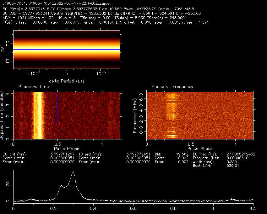
You can see that the pulse profile looks vertical in both frequency and time (although they already were).
It also outputs an estimated period and DM in the plot and in the pdmp.posn and pdmp.per.
BC is barycentric which is based on the centre of the solarsystem and what is used by pulsar ephemerises TC is topocentric which is based on the earth’s position. Because the aparent/observed period is different depending on the position of the earth as it orbits the as the change in distance and relative speed causes an effect similar to the doppler effect. Pulsar software will convert barycentric period to topocentric period for you so always give it the barycentric period.
Decimating
You can decimate or scrunch your data along the time, frequency and polarisation axis. A major benfit of this is that it makes the files much smaller. Another benefit is that the files will be in an easier format to make ToAs later on (convered in future lessons).
The wording used commonly used to describe how the data has been decimated is “nchan” for number of frequency channels and “nsub” for number of time sub-integrations.
The following command demonstrates how to use pam
pam --setnchn <nchan> --setnsub <nsub> <-p> -e <nchan>ch<-p>p<nsub>t.ar <archive_file>
where you use -p if you want to polarisation scrunch and -e <nchan>ch<-p>p<nsub>t.ar is my personal preference of how to label the file to make it clear how it has been decimated.
So for example if you wanted 16 frequency channels and 8 time sub-integrations:
pam --setnchn 16 --setnsub 8 -e 16ch4p8t.ar J1903-7051_2022-07-17-22:44:02_zap.ar
Organisation
Dealing with data can be a bit confusing and you may get a bit lost if you don’t keep your data organised. The following is a few tips that will hopefully make your life easier.
- Use good names for your files. Verbose long names are better than short confusing names. You should include the pulsar name and the date it was observed as well as other things like if you have removed RFI and if and how you have decimated it.
- Make a script to automate your work. Once you have worked out how to process your data, you can make a script that will run all those commands for you which will save you time and make sure you don’t forget a step.
- Use a kanban board (to do list) to track your processing. If you have a lot of data to process it may start to ger hard to keep track of what you have and haven’t done. One way to make this easier is to use a kanban board like Trello (see this lesson on how to use it)
- Take notes on the commands you used. Taking notes will make it clearer what steps you took and may help you if you forgot how to use a command. An easy way to do this is to dump the last 100 commands you ran with the following command
history | tail -n 100 > my_commands.txt
Done!
Our data has been cleaned, checked and formated so we are ready to start making ToAs and do some timing!
Key Points
There are different types of pulsar data and different ways to process them
Removing RFI can be difficult but will significantly improve your data
Keeping your data organised will make your work easier